
Everybody knows the multiplication tables that we have learnt at school but less people knows a fascinating aspect of them. At first glance, the multiplication tables is an elementary subject, not exactly exciting, and yet we are going to discover the hidden face of the multiplication tables that will surely surprise you.
The aim of this post is to make a computer program written in Golang and SDL which is visualizing the multiplication tables. So firstly, we will need a graphical representation of the multiplication tables instead of an algebraic representation as the following table.
| x | 0 | 1 | 2 | 3 | 4 | 5 | 6 | 7 | 8 | 9 |
|---|---|---|---|---|---|---|---|---|---|---|
| 0 | 0 | 0 | 0 | 0 | 0 | 0 | 0 | 0 | 0 | 0 |
| 1 | 0 | 1 | 2 | 3 | 4 | 5 | 6 | 7 | 8 | 9 |
| 2 | 0 | 2 | 4 | 6 | 8 | 10 | 12 | 14 | 16 | 18 |
| 3 | 0 | 3 | 6 | 9 | 12 | 15 | 18 | 21 | 24 | 27 |
Graphical representation
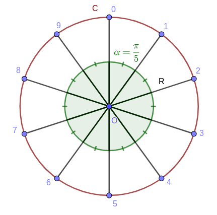
Let’s take a circle C of radius R centered at O:(0,0). Take an arbitrary number of points M from 0 to M-1, fairly distributed on the circle C. The alpha angle between each point from the center O is  , for instance if
  . We will represent the numbers cyclically on the circle. For example the numbers 10, 20, … will be on the point zero, the numbers 11, 21, … on the point one, etc … In mathematics this branch is called modular arithmetic. In our example, we can say that we represent the numbers modulo 10. By convention the modulo’s symbol is %.
Now that we are able to represent the multiplication tables on the circle. Let’s take a multiplication  where N is the multiplied number, T is the table number, R the result and a modulo M. The principle is simple: to represent this multiplication graphically, we have to draw a line between the points N and R % M.
For example, let’s start by the multiplication table of 2 module 10.
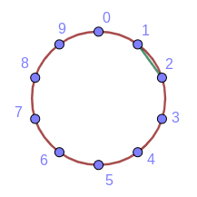
Line from 1 to 2.
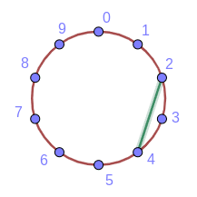
Line from 2 to 4.

Line from 5 to 0.

Line from 7 to 4.
Here we go, we can see the final representation of the multiplication table of 2 modulo 10 with the following animation.
Now that we are able to graphically represent a multiplication table, we need to have a system of configuration in order to know what we want to represent. As we will see, we will need to represent a combination of many tables and modulos to see the fascinating hidden face of the multiplication tables.
Configuration
By definition a configuration is the inputs with the tables and the modulos which have to be sequentially computed and graphically represented. By convention:
- The surface is the container of the table graphical representation.
- 1 table T and 1 modulo M is called a tuple (T, M).
- We always browse the tables first, then the modulos, each tuple representation is called a frame.
- The combinations of tuples are allowed, eg: (T:2, M:[10,11]) is a combination of 2 tuples (T:2, M:10) and (T:2, M:11)
- We use the JSON format to write a configuration.
- Between each frame we clean the surface and we have a timelapse which is a settable option.
For example if we want to visualize the simple previous illustration: (T:2, M:10):
{
    "table": {
        "values": [ 2 ]
    },
    "modulo": {
        "values": [ 10 ]
    }
}
If we want to graphically represent the following 4 tuples: (T:[2,3],M:[10,11]). As we mentioned by convention, the evaluation will be: (T:2, M:10), (T:2, M:11), (T:3, M:10), (T:3, M:11). We always evaluate the tables first.
{
    "table": {
        "values": [ 2, 3 ]
    },
    "modulo": {
        "values": [ 10, 11 ]
    }
}
An other syntax is allowed to facilitate the write of the configuration, for example if we want to compute the table of [2,3] with modulo [10.1, 10.2, 10.3, … 20].
{
    "table": {
        "values": [ 2, 3 ]
    },
    "modulo": {
        "from": 10,
        "to": 20,
        "step": 0.1
    }
}
Then we have a system of configuration to have the proper inputs, let’s take a look on the program which will draw the graphical representation of theses configurations.
Program
Firstly we have to parse the JSON configuration. In Golang, it is really simple with the package encoding/json. You just have to map a Golang structure with the JSON structure.
type v struct {
	Values []float64 `json:"values"`
	From   float64   `json:"from"`
	To     float64   `json:"to"`
	Step   float64   `json:"step"`
}

type input struct {
	Table  v `json:"table"`
	Modulo v `json:"modulo"`
}
To get the configuration, you just have to read a file and unmarshal the content into an instantiation of this structure.
var I input
data, err := ioutil.ReadFile(opts.input)
if err != nil {
	panic(err)
}
json.Unmarshal([]byte(data), &I)
Next step is to process the coordinates of the points and draw the lines into the circle. A little mathematical reminder can be useful here. As we mentioned above, with a modulo M, we have M points fairly distributed. So the angle between each line is . In classical trigonometry, the origin point is on the xAxis at coordinates (X:1,Y:0) but in our case we want this point at (X:0,Y:1) so we do an anticlockwise rotation of  , this is why x is calculated with the sine and y with the cosine.
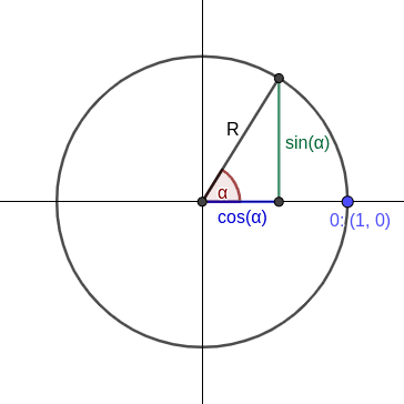
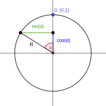
If N is the nth point of the circle then:
(1) 
func get(alpha, N float64) (float64, float64) {
	x := math.Sin(N*alpha) * R
	y := math.Cos(N*alpha) * R
	return x, y
}
We are able to get the coordinates of a point, we have to draw the line between 2 points (x1:N) and (x2:R) from the multiplication 
func line(alpha, N, T, M float64) {
	R := math.Mod(T*N, M)
	x1, y1 := get(alpha, N)
	x2, y2 := get(alpha, R)
	// Draw the line between x1 and x2
}
To end, we have to loop on each frame of a configuration (pseudo code below, full code available here):
foreach table T {
  foreach modulo M {
    // clean the surface
    alpha := (2 * PI) / M
    for N from 1 to M {
       line(alpha, N, T, M)
    }
    // refresh the surface
  }
}
Hidden face
Let’s play with the program to see the hidden face of the multiplication tables ! A lot of predefined configurations are available. The following command is an example on how to run the program (reminder: github repository).
❯❯❯ # example of run with (T:2, M:10)
❯❯❯ go run . --input configurations/2mod10.json --timelapse 10 # millisecond
Let’s start with the three following simple configurations:
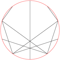
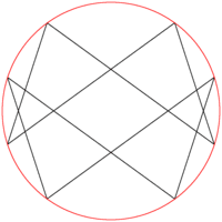
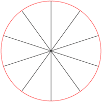
Three more complex configurations with geometric specificity:
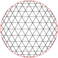
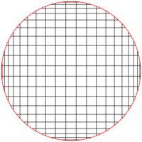
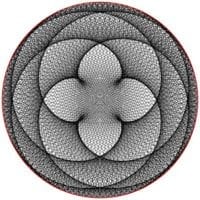
(T:399, M:993)
WOW ! It is fascinating to see with a simple rule, as the multiplication table, that we can produce such optical illusions. For the time being, we only represented some static configurations, by static I mean 1 table, 1 modulo and 1 frame. Let’s take a look at some simple beautiful configurations with multiples frames.
This first configuration shows the multiplication tables from 2 to 9 with 300 points (modulo 300) and a step of 0.1. The time-lapse is set to 40 millisecond between each frame.
Surprise ! We have N-1 flower petals for the table of N.
This second configuration shows the multiplication table of 2 from 10 to 100 points with a step of 0.1. The time-lapse is set to 1 millisecond between each frame.
Look that ! The curves appear from nowhere !
To conclude, my favorite configuration, one of the multiplication table that I’m considerate as the most beautiful and complex optical illusion ! It is the table of 366 to 375 with a step of 0.01 and a module 855.
Isn’t it beautiful and magical to see this complexity coming from the simplicity of multiplication tables?
I hope you will play with the program to discover new configurations and share with me the bests you find !
If you have loved this post, you may be loved the pi computation algorithms.
Feel free to leave a message for any questions or suggestions, I’ll be more than happy to answer, you can also contact me at: contact@algomaths.tech
Thomas Joly