The purpose of this post is to explain, illustrate and code different PI computation algorithms from antiquity to the present. We will see that π is everywhere like in the physics collisions, in pure mathematical series or even in the randomness.
The number π is a mathematical constant. It is defined as the ratio of a circle’s circumference to its diameter.  . It appears in many formulas in all areas of mathematics and physics. It is approximately equal to 3.14159. It has been represented by the Greek letter “π” since the mid-18th century and is spelled out as “pi”. It is also referred to as Archimedes’ constant.

π is irrational, that is, it cannot be written as a fraction of two integers and its decimal writing is neither finite nor periodic. It also means that Pi’s digits are not predictable. π is also a transcendental number, not being the solution of any equation with rational coefficients.

π is a mysterious and fascinating number, here are some crispy anecdotes:
- The best known approximate decimal value of π currently has around 1241 billion digits.
- There is a club of people who know more than 1000 Pi decimal places by heart: The 1000-club.
- The officially recognized π memorization record is 67,890 digits, held by Lu Chao, a young Chinese graduate. It took him 24 hours and 4 minutes to recite Pi’s first 67,890 decimal places without error.
- It was used for the construction of the pyramids.
- Am I in PI ? allows you to find a date of birth hidden in the decimal places of π.
In this post, we will talk about precision/accuracy of approximation with different PI computation algorithms. It is the number of exact significant digits based on the following reference from https://oeis.org/A000796.
const (
    Pi  = 3.14159265358979323846264338327950288419716939937510582097494459
)
For instance 3.149999 has an accuracy of 3.
Let’s begin at the beginning !
Antiquity – Triangles PI estimation
One of the first recorded PI computation algorithms for rigorously calculating the value of π was a geometrical approach using polygon, devised around 250 BC by the Greek mathematician Archimedes. This polygon algorithm dominated for over 1,000 years, and as a result π is sometimes referred to as “Archimedes’ constant”. In our case, we will illustrate a derivative algorithm from Archimedes with triangles instead of polygons, but the principle stays the same.
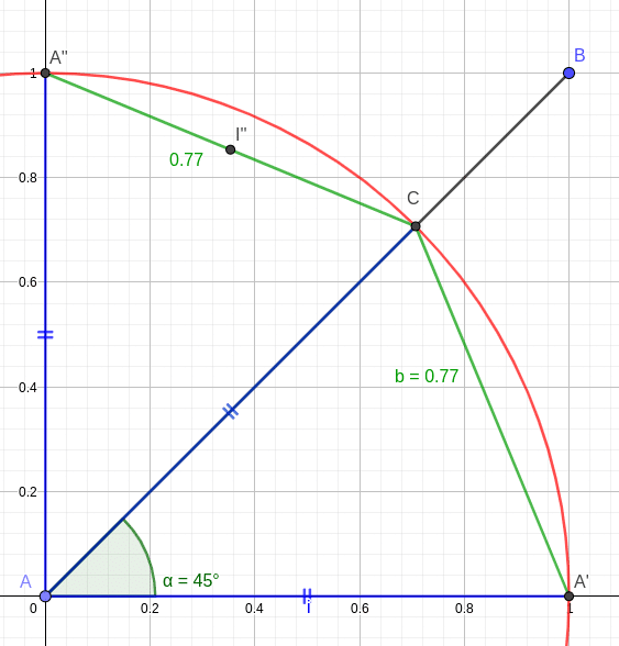
The aim is to divide a circle of radius 1 into N triangles as the illustration. For instance, we divide the circle into 8 triangles. Each triangle is an isosceles triangle with an apex angle of 45º ( ). For example the angle
  .
.
We measure with a ruler the base of the triangle b = [A’,C] = 0.77. Furthermore, π was commonly defined as the ratio of a circle’s circumference C to its diameter D: . The circumference C can be approximate by b multiply N. So, we can approximate π by  . If we trend the number of triangles to infinity, we will have a more accuracy estimation of π, which already illustrates the “analytical” character of π.
Around 150 AD, Greek-Roman scientist Ptolemy, in his Almagest book, gave a value for π of 3.1416, which he may have obtained from Archimede.
The following code estimates π, given in argument the number of triangles. Previous animations are done with Golang and SDL. The full code is available here.
// emulate a manual measure with a ruler of the triangle base
func measureBase(a, theta float64) float64 {
	return 2 * a * math.Cos(common.Radian(theta))
}

func trianglePIEstimation(triangles float64) float64 {
	alpha := 360.0 / triangles
	theta := (180.0 - alpha) / 2.0
	base := measureBase(radius, theta)
	circumference := base * triangles
	return circumference / (2 * radius)
}
Let’s make a leap forward of 1400 years.
Leibniz formula – Mathematical series
Maybe the most elegant mathematical formula (alternating series) to approximate π discovered by Leibniz in 1674:

But this series converges so slowly that to calculate π with an accuracy of six decimal places it takes almost two million iterations. The full code is available here.
func leibniz(iteration int) float64 {
	n := 0
	sum := 0.0
	numerator := 1.0
	denominator := 1.0

	for {
		sum += numerator / denominator
		numerator *= -1
		denominator += 2
		n++
		if n == iteration {
			break
		}
	}
	return sum * 4.0
}
Approximate fractions – Simplest computation
The fractions are the simplest process used to approximate π:
| numerator | denominator | PI estimation | accuracy |
|---|---|---|---|
| 3 | 1 | 3 | 1 |
| 22 | 7 | 3.14285714286 | 3 |
| 333 | 106 | 3.14150943396 | 5 |
| 355 | 113 | 3.14159292035 | 7 |
| 103993 | 33102 | 3.14159265301 | 9 |
The first Hewlett-Packard calculators (eg HP-25) did not have a key for π, and the recommended user manual give the following fraction
, which is very easy to memorize.
 , which is very easy to memorize.
By comparison, the last fraction has more accuracy than the Leibniz formula computation with 100,000,000 iterations.
Let’s take a look on the modern mathematical formulas to approximate PI as efficient as possible.
Machin-like formula – Efficiency
In mathematics, Machin-like formulas are a popular technique for computing π to a large number of digits. They are generalizations of John Machin’s formula from 1706:

func johnMachin() float64 {
	n1 := 4 * math.Atan2(1, 5)
	n2 := math.Atan2(1, 239)
	return 4 * (n1 - n2)
}
Full code is available here. The search for effective Machin formulas is now done systematically using computers. One of the most efficient Machin type formulas currently known to calculate π are the Hwang Chien-Lih in 1997:

There are other formulas that converge more quickly to π, such as Ramanujan’s formula, but they are not Machin-like formula and it is not really interesting for the post (pure mathematics, not PI computation algorithms), but I wanted you to know that this exists.
After pure mathematical methods, let’s see how we can find an approximation of PI with the random!
Monte-Carlo – Random is the key
Monte Carlo methods or Monte Carlo experiments, are a broad class of computational algorithms that rely on repeated random sampling to obtain numerical results. The underlying concept is to use randomness to solve problems that might be deterministic in principle. Monte Carlo method can be applied to approximate the value of π.
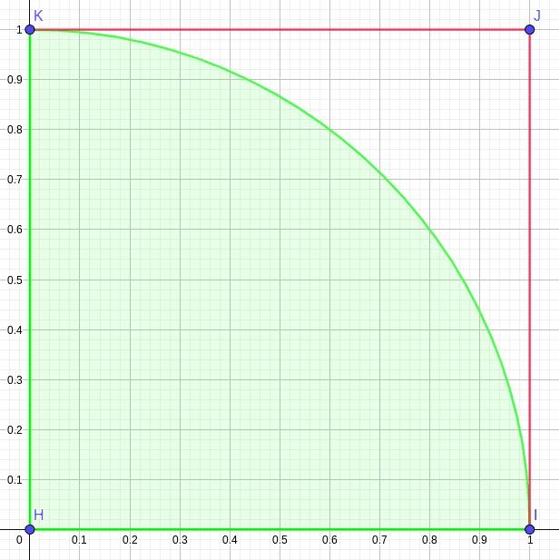
We consider in a plane the square SQ of vertices (H,I,J,K) with: H:(0,0), I:(1,0), J:(1 1) and K:(0,1).
We also consider a circle C of origin H:(0,0) and radius R=1, and a sector SC of circle C (H,I,K).
Let M be a point of coordinates ![(x, y), \text{where } x,y \in [0,1]](https://b2122273.smushcdn.com/2122273/wp-content/ql-cache/quicklatex.com-c43310166d8f18e86a1225c1d9888cf2_l3.png?lossy=1&strip=1&webp=1 "Rendered by QuickLaTeX.com") . We randomly draw the values of x and y between 0 and 1 according to a uniform law. So, the point M is in the sector circle SC , if and only if,
. We randomly draw the values of x and y between 0 and 1 according to a uniform law. So, the point M is in the sector circle SC , if and only if,  .
.
The probability that the point M belongs to the disk is  . Since the quarter of the disk is of surface
  , and the square SQ that contains it is of surface
  . If the probability is a continuous uniform distribution, the probability of falling into the quarter disc is
  .
.
func monteCarlo(iteration int) float64 {
	r := 0
	n := 0
	for {
		x := rand.Float64()
		y := rand.Float64()
		if x*x+y*y <= 1 {
			r++
		}
		n++
		if n == iteration {
			break
		}

	}
	return 4 * float64(r) / float64(n)
}
By making the ratio of the number of points in the disc to the number of prints, we obtain an approximation of the number if the number of prints is large.
This method is maybe the least precise approximation of π but it is magic to find one of the PI computation algorithms with a random experiment. With a perfect continuous uniform distribution, the estimation should be better. Let’s see the next experiment which giving an exact approximation of π based on physics laws.
Blocks collisions – Physics conspiracy
Sometimes mathematical and physics conspire in ways that feel too good to be true. Let’s play a strange sort of mathematical croquet.
Let’s take two sliding blocks B1 and B2 and a wall W. The block B1 starts by coming in at some velocity v1 from the right and mass m1, while the second block B2 starts out stationary with a velocity v2 equals to 0 and a mass m2. Being overly-idealistic physicists, let’s assume that there is no friction and that all collisions are perfectly elastic, which means no energy is lost. The goal will be to count how many collisions take place.

By deduction/convention, let’s say:
- We note a collision between 2 entities E1 and E2: E1 <> E2.
- A collision can be done between both blocks or between the block B2 and the wall W.
- The blocks can slide infinitely to the right.
- A velocity from right to left is negative.
- A velocity from left to right is positive.
The simplest case is when both blocks have the same mass. B1 hits B2, transferring all of its momentum. Then B2 bounces off the wall, then it transfers all of its momentum back to the block B1, which goes off to infinity. For instance, we can resume this setup :  .
.
Now we will see a mathematical robust solution to find the number of collisions for any  inputs. Velocities are constant for the setup
  .
.
Two physics laws have to be respected for blocks collisions:


We are assuming that:


If we put x and y in the previous equations, we get the following system of equation:
(1) 
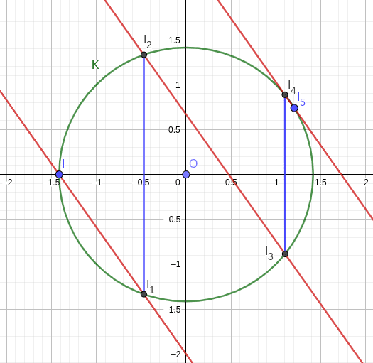
- The first one is a line with equation:
- The second one is a circle centered at {0,0} with radius . Because the circle, with initial conditions , has to pass by the point .

 . Because the circle, with initial conditions
  .
.A := math.Sqrt(m1) B := math.Sqrt(m2) R := A
A, B and R will be constant for each iteration (collision) because the mass are constant. The algorithm to find the next velocities after each collision is pretty simple:
- Increment collisions (between the both blocks).
- Compute C from the conversation of momemtum :
- Deduce the new line equation
- Find the new intersection between line and circle
- Update velocities:
- If v2 < 0 then increment collisions (between B2 and W).
- If v1 > v2 && v1 > 0 then stop the loop: no more collision.


Let’s take an example with  . We have a circle K of radius
  and an initial point
  .
.
| iteration | v1 | v2 | collision | C | line equation | intersection | number of collisions |
|---|---|---|---|---|---|---|---|
| 0 | -1 | 0 | B1 <> B2 | -(2 * - 1 + 1 * 0) = 2 | eq1: 1.41.x + y + 2 = 0 | I1 = (-0.47, -1.33) | 1 |
| 1 | -0.33 | -1.33 | B2 <> W | NC | NC | I2 = (-0.47, 1,33) | 2 |
| 2 | -0.33 | 1.33 | B1 <> B2 | -(2 * -0.33 + 1 * 1.33) = -0.67 | eq2: 1.41.x + y - 0.67 = 0 | I3 = (1.1, -0.89) | 3 |
| 3 | 0.78 | -0.89 | B2 <> W | NC | NC | I4 = (1.1, 0.89) | 4 |
| 4 | 0.78 | 0.89 | B1 <> B2 | -(2 * -0.78 + 1 * 0.89) = -2.45 | eq3: 1.41.x + y - 2.45 = 0 | I5 = (1.20, 0.74) | 5 |
| 5 | 0.85 | 0.74 | No collision | NC | NC | NC | 5 |
The following code computes the number of collisions. Full code is available here.
	for {
		collisions++ // blocks collision
		C := -(opts.m1*v1 + opts.m2*v2)
		x, y := common.GetIntersections(A, B, C, R)
		v1 = x / math.Sqrt(opts.m1)
		v2 = y / math.Sqrt(opts.m2)
		if v2 < 0 {
			collisions++ // wall collision
			v2 = -v2
		}
		if v1 > v2 && v1 > 0 {
			break // no more collision
		}
	}
I use the algorithm from this post to find intersections between circle and line (common.GetIntersections).
Now we are able to resolve the whole problem of blocks collisions. What about if that first block has 100 times the mass of the second one ?
lunamath ❯❯❯ go run pi/collisions/collisions.go --m1 100 --m2 1
collisions: 31
What about if that first block has 10.000 times the mass of the second one ?
lunamath ❯❯❯ go run pi/collisions/collisions.go --m1 10000 --m2 1                                                                                                                                               pi estimation physics collisions
collisions: 314
If it was 1.000.000 times the mass of the second, then again, with all our idealistic conditions:
lunamath ❯❯❯ go run pi/collisions/collisions.go --m1 1000000 --m2 1
collisions: 3141
Perhaps you see the pattern here, thought it is forgivable if you don’t see since it defies all expectations. When the mass of the first block is some power of 100 times the mass of the second block, the number of collisions will have the same digits as the beginning of π…. Amazing!!!!

This fact was originally discovered by the mathematician Gregory Galperin in 1995, and published in 2003. The youtube channel 3Blue1Brown made three videos on that topic, very well explained (here).
This method is maybe the most elegant method of PI computation algorithms but not really the most efficient. For example, to calculate only 20 digits of PI, the first block would have 100 billion, billion, billion, billion times the mass of the second block  . If the second block was 1kg means the first block has a mass of 10 times that of the supermassive black hole at the center of the milky way.
What next ?
I loved to discover these different PI computation algorithms and I hope you loved too ! It was my first experience with mathematical post and I will do it again with the golden ratio for example. Don’t hesitate to read my other posts with many interesting algorithms like the expectiminimax with the bot 2048 or the backtracking with the sudoku solver.
Feel free to leave a message for any questions or suggestions, I’ll be more than happy to answer, you can also contact me at: contact@algomaths.tech
Thomas Joly